| Cost function | γ (attractiveness) | β (deterrence) | β units | R² | RMSE |
|---|---|---|---|---|---|
| Power | 0.114 | 0.076 | dimensionless (elasticity) | 0.1163 | 4.121 |
| Exponential | 0.116 | 0.000023 | per metre | 0.1168 | 4.120 |
Retail Location Optimisation via Spatial Interaction Modelling: A Case Study of the Borough of Havering
Retail Optimisation
Urban Simulation
SIM
This study explores the use of a production-constrained spatial interaction model to evaluate two candidate supermarket locations in the London Borough of Havering.
Objective
This study applies a production-constrained spatial interaction model to evaluate two candidate supermarket locations in the London Borough of Havering. A poisson log-linear GLM with exponential distance decay was calibrated using 80,604 customer trips across 775 local areas and 56 existing stores.
By comparing two potential sites, the model reveals that footfall was more sensitive to overall location and accessibility than store size, with Location A drawing 11% more predicted traffic than Location B due to its central reach, which widens if travel costs rise. However, Location B outperforms Location A in local walkability, with over 1,700 more residents living within a 15-minute walk. These results highlight the strategic tension in retail location analysis, forcing decision makers to weigh macro-level catchment against micro-level pedestrian accessibility.
2. Spatial Interaction Models
Spatial interaction models are used to predict flows (e.g. trips, trade, migration) between origins \(i\) and destinations \(j\) as a function of the characteristics at each location and the cost of travelling between them. The simplest gravity model, as formalised by Wilson (1971), assumes that interaction is proportional to the “mass” at each location and inversely proportional to the separation between them.
2.1 Introduction to Spatial Interaction Models
2.1.1 Unconstrained (gravity) model
The basic form is the unconstrained gravity model, where only total flows are conserved. This is commonly used in trade or migration modelling where neither origin nor destination totals are known in advance.
\[ T_{ij} = KO_i^{\alpha} D_j^{\gamma} f(c_{ij}) \tag{1} \]
where \(T_{ij}\) is the predicted flow from origin \(i\) to destination \(j\). \(O_i\) and \(D_j\) represent origin and destination parameters (e.g. population or jobs), and \(c_{ij}\) is distance or travel cost. \(f(c_{ij})\) is a deterrence or cost function that captures decay with either a power function \(c_{ij}^{-\beta}\) or an exponential function \(e^{-\beta c_{ij}}\), where \(\beta\) is the distance decay parameter — a larger \(\beta\) means people are much less willing to travel far. \(K\) is a scaling constant, while \(\alpha\) and \(\gamma\) are elasticity parameters calibrated from data. \(\alpha\) governs how strongly origin size translates to flow generation, and \(\gamma\) models how strongly destination attractiveness influences flows. For example, a larger \(\gamma\) means larger stores draw disproportionately more people. When \(\alpha = \gamma = 1\), the model reduces to the standard gravity form.
2.1.2 Production-constrained model
The production-constrained (origin-constrained) model imposes \(\sum_j T_{ij} = O_i\), ensuring total outflows from each origin match observed production through balancing factor \(A_i\). This specification is typically applied in retail location analysis and transport trip distribution, where the number of trips originating from each zone is known but destination choice is to be modelled.
\[ T_{ij} = A_i O_i D_j^{\gamma} d_{ij}^{-\beta}, \quad \text{where} \quad A_i = \frac{1}{\sum_j D_j^{\gamma} d_{ij}^{-\beta}} \tag{2} \]
2.1.3 Attraction-constrained model
The attraction-constrained (destination-constrained) model imposes \(\sum_i T_{ij} = D_j\), ensuring total inflows into each destination match observed flows through balancing factor \(B_j\). This specification is typically applied where destinations have fixed capacities, such as migration to cities with a fixed housing stock or hospital allocation with fixed bed counts.
\[ T_{ij} = B_j O_i^{\alpha} D_j d_{ij}^{-\beta}, \quad \text{where} \quad B_j = \frac{1}{\sum_i O_i^{\alpha} d_{ij}^{-\beta}} \tag{3} \]
2.1.4 Doubly-constrained model
Finally, the doubly-constrained model is used when both origin and destination totals are known. Both \(\sum_j T_{ij} = O_i\) and \(\sum_i T_{ij} = D_j\) must hold simultaneously, enforced by coupled balancing factors \(A_i\) and \(B_j\). As both totals are fixed, the elasticities \(\alpha\) and \(\gamma\) are no longer free parameters and \(O_i\), \(D_j\) enter linearly. Since \(A_i\) and \(B_j\) are mutually dependent, they are solved iteratively. This model is well-suited to commuting flows, where both residential population and workplace employment totals are known.
\[ T_{ij} = A_i B_j O_i D_j d_{ij}^{-\beta}, \quad \text{where} \quad A_i = \frac{1}{\sum_j B_j D_j d_{ij}^{-\beta}} \quad \text{and} \quad B_j = \frac{1}{\sum_i A_i O_i d_{ij}^{-\beta}} \tag{4} \]
2.2 Fitting and Calibrating Spatial Interaction Models
The production-constrained model is adopted for this analysis, given that we know the residential population in each of the 775 Output Areas (OAs) in Havering, and wish to predict how these populations distribute their trips across 56 existing supermarkets (i.e. we don’t know destination totals). The attractiveness of each store can be measured by its floor area (m²), and the cost is the road network distance.
We test both a power and an exponential cost function to model deterrence.
| Cost Function | Formula | Behaviour |
|---|---|---|
| Power (inverse) | \(f(d) = d^{-\beta}\) | Slow initial decay, heavy tail. People occasionally travel far |
| Exponential | \(f(d) = e^{-\beta d}\) | Rapid decay. Interaction drops off sharply with distance |
We specify the production-constrained model as a Poisson regression by taking logs of the right-hand side of Equation \((2)\) and assuming these are logarithmically linked to the Poisson-distributed mean (\(\lambda_{ij}\)) of the \(T_{ij}\) variable:
\[ \text{Power function:} \quad \lambda_{ij} = \exp(\alpha_i + \gamma \ln D_j - \beta \ln d_{ij}) \tag{5} \]
\[ \text{Exponential function:} \quad \lambda_{ij} = \exp(\alpha_i + \gamma \ln D_j - \beta d_{ij}) \tag{6} \]
Here \(\alpha_i\) are origin fixed effects estimated for each OA, which absorb the balancing factor \(A_i O_i\) and directly enforce the production constraint \(\sum_j \hat{T}_{ij} = O_i\) for every origin exactly.
We obtain the regression outcomes in Table 1.
Both models yield similar goodness-of-fit, with the exponential form marginally better. The low \(\gamma \approx 0.114\) indicates that store size has only a modest effect on store choice. The low \(\beta\) values indicate a relatively flat distance decay, meaning that people in Havering are more willing to travel, consistent with car-dependent suburban retail patterns. The \(R^2\) of \(\approx 0.12\) is modest but expected given the sparsity of the observed flow matrix.
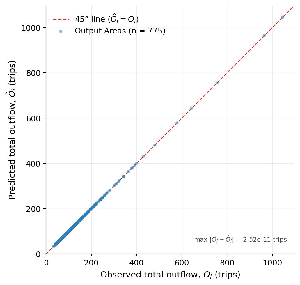
Flow conservation is guaranteed structurally by the balancing factor \(A_i\), defined as:
\[ A_i = \frac{1}{\sum_j D_j^{\gamma} \, d_{ij}^{-\beta}} \]
which ensures that \(\sum_j \hat{T}_{ij} = O_i\) for all \(i\). This is confirmed empirically in Figure 1.
3. Scenario Analysis
3.1 Assessment of Two Candidate Supermarket Locations
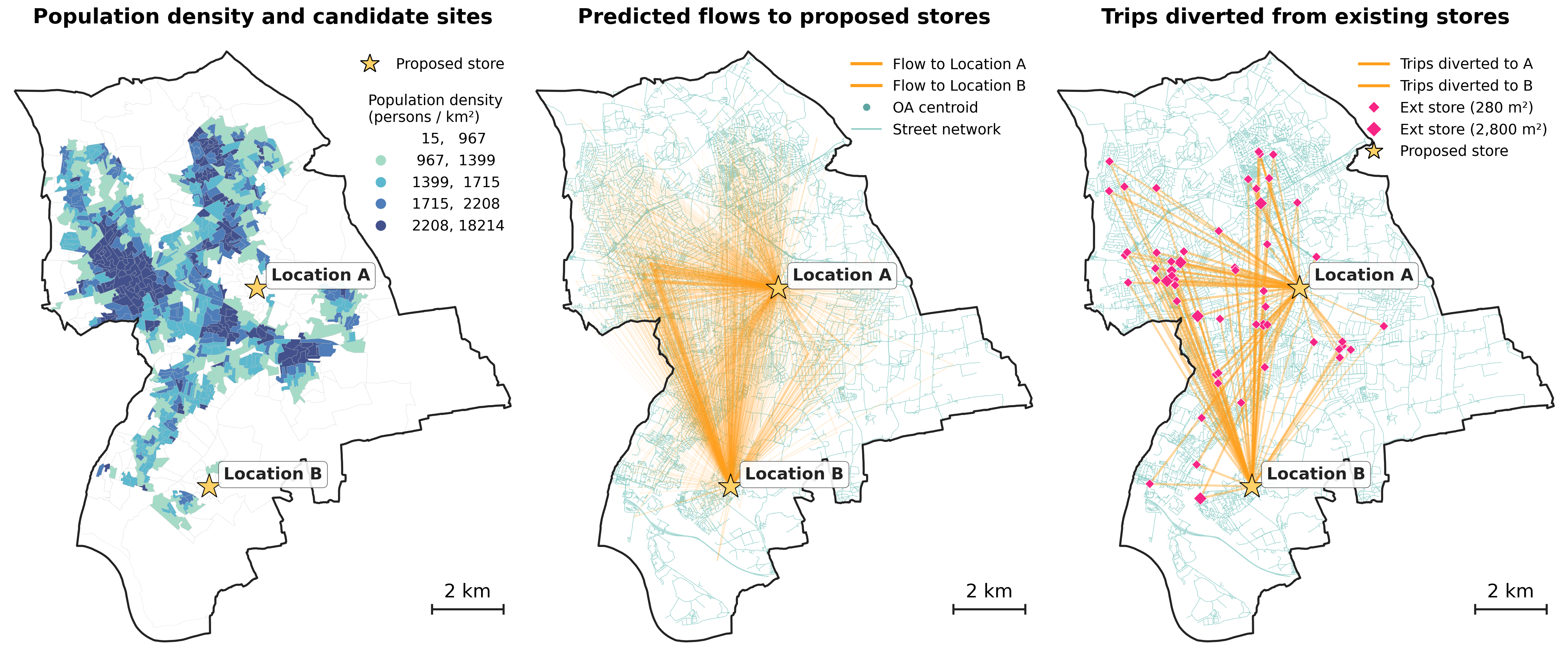
Two candidate sites in the London Borough of Havering are evaluated. Location A (E00011326) is sited centrally, where population is more concentrated but competition is stricter. Location B (E00011710) sits at the Southern periphery with less surrounding competition (Figure 2). The site assessment is undertaken under two scenarios, each introducing a single new store into the destination set independently.
We undertake simulation for two store sizes (\(\text{Small} = 280\text{ m}^2, \text{Large} = 2,800\text{ m}^2\)) to evaluate the sensitivity of the results to store size.
The negative exponential cost function is adopted. Access to supermarkets is highly localized, as individuals exhibit strong sensitivity to distance when carrying purchases home, a pattern well-captured by the exponential form’s rapid spatial decay (devries2004?). Unlike the long-tailed power function, which overestimates the relevance of distant supermarkets, the exponential model better reflects routine suburban access constraints. This conceptual fit is confirmed empirically, yielding superior goodness-of-fit (\(R^2 = 0.1168\), \(\text{RMSE} = 4.120\)) compared to the power model (\(R^2 = 0.1163\), \(\text{RMSE} = 4.121\)).
The calibrated \(\hat{\gamma}\) and \(\hat{\beta}\) are held fixed from the calibration stage; only \(A_i\) is recomputed to accommodate the expanded destination set, with flow conservation verified after each run.
Summary of Results
| Metric | Small A | Small B | Large A | Large B |
|---|---|---|---|---|
| Total flow (trips) | 1,368 | 1,228 | 1,782 | 1,605 |
| Mean weighted distance | 4,397 m | 8,819 m | 4,391 m | 8,743 m |
| Mean market share | 1.72% | 1.55% | 2.25% | 2.02% |
Location A (E00011326) is the stronger investment in both scenarios. It attracts 11% more flow than Location B, as the exponential cost function penalises Location B’s peripheral position (mean customer distance ~4.4 km vs ~8.8 km for B). Location B (E00011710) sits on the southern periphery of the borough, where the surrounding population is sparse and most residents face longer distances to reach it.
We observe a modest size effect (\(\gamma = 0.11\)). Scaling from \(280\ m^2\) to \(2{,}800\ m^2\) increases predicted flow by approximately 30%, consistent across both locations, as \(\gamma\) enters the model uniformly regardless of site.
One limitation is that only flows from within Havering are redistributed to the proposed supermarkets. In reality, Location B’s position on the southern boundary means that OAs outside Havering’s southern edge fall within its natural catchment but are excluded from the model, which may cause its predicted flows to be slightly underestimated relative to Location A.
3.2 Assessment of Sharp Increase in Transport Costs
Assuming a sharp increase in transport cost arising from a congestion and fuel surcharge, residents would be more reluctant to travel long distances. This could translate to a sharper distance decay function. We explore what happens when \(\beta\) increases by 50% and 100%. The calibrated baseline \(\beta = 0.000023\) per meter implies that a journey of 5 km is discounted by a factor of \(e^{-0.000023 \times 5000} \approx 0.89\) relative to a journey of zero distance. Doubling \(\beta\) to \(0.000046\) increases this penalty to \(e^{-0.000046 \times 5000} \approx 0.79\), meaning longer trips become meaningfully less attractive under the shock scenario.
The sensitivity analysis reveals an asymmetric response to transport cost increases. As \(\beta\) increases by 50% and 100%, Location B’s predicted flows decline consistently across both size scenarios, while Location A’s flows increase marginally (Figure 3). This reflects the mechanics of the production-constrained model: as \(\beta\) rises, the exponential decay penalises Location B’s peripheral position more severely, and the balancing factor \(A_i\) redistributes those lost trips to closer alternatives. The mean weighted distance to Location A also falls slightly under higher \(\beta\) (4,416 m → 4,379 m), confirming that its catchment becomes more localised and efficient under cost pressure.
| Scenario | β (baseline) | 1.5β | 2β | Δ vs baseline | Δ % |
|---|---|---|---|---|---|
| Small A | 1,382 | 1,389 | 1,395 | +13 | +0.9% |
| Small B | 1,253 | 1,201 | 1,152 | -101 | -8.1% |
| Large A | 1,796 | 1,805 | 1,813 | +17 | +0.9% |
| Large B | 1,629 | 1,561 | 1,498 | -131 | -8.0% |
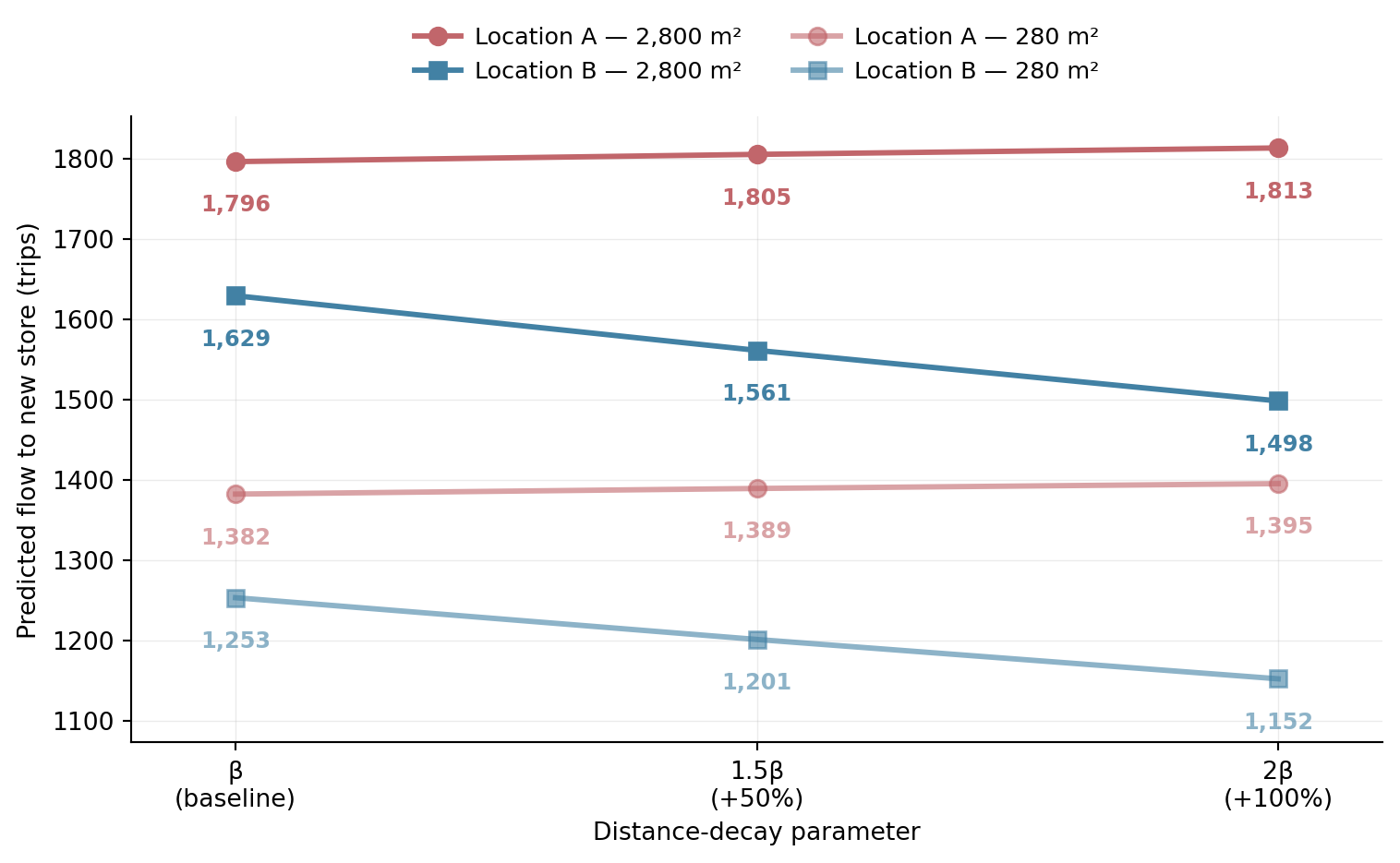
Location A remains the recommended investment under the transport cost increase scenarios. Its relative advantage over Location B widens as costs increase. This finding is robust to the cost shock assumption.
3.3 Walkability Access within 15-min catchment
To determine walkability access to the proposed supermarket, we compute the number of residents whose Output Area centroid lies within a 15-minute walking catchment of each candidate location. We adopt TfL’s assumed walking speed of 1.3 m/s (TfL, 2025b), giving a maximum walking distance of:
\[d_{walk} = 1.3 \times 60 \times 15 = 1{,}170 \text{ m}\]
We can use the road network distance from each OA centroid to the candidate store node, computed via OSMnx shortest path lengths, to determine which OAs fall within this threshold. Figure 4 illustrates the 15-minute walking catchment for each candidate site. The top row shows the accessible road network within 15 min for both locations and Output Areas that fall within. The bottom row shows the resident population as dot density within those same areas.
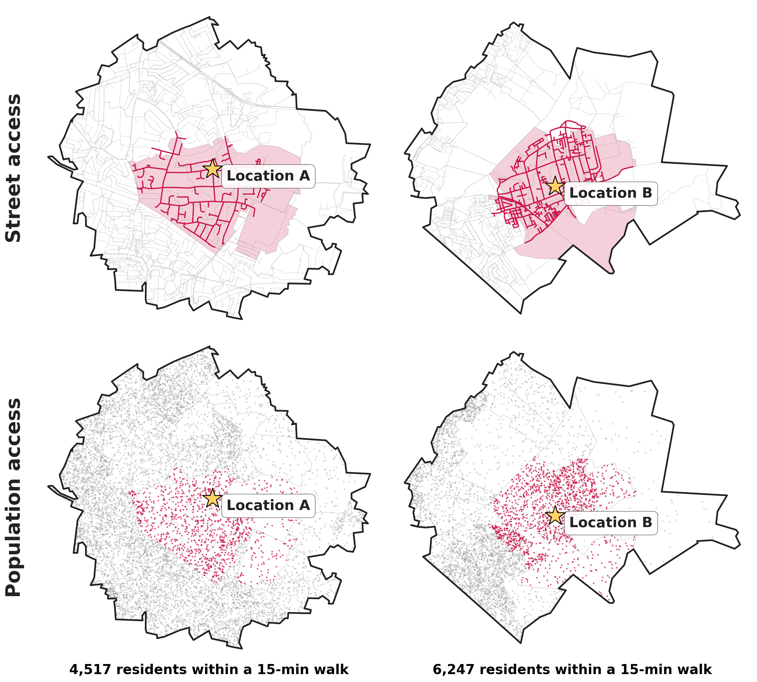
Within a 15-minute walk, Location B serves a visibly larger accessible population (6,247 residents across 18 OAs) compared to Location A (4,517 residents across 13 OAs), as seen by the thicker dot density in Figure 4.
This reversal reflects an important distinction between local walking access and borough-wide trip attraction. Location B’s southern catchment, while peripheral in the context of Havering as a whole, sits within a relatively densely populated residential area at close road network distances. Location A, despite attracting significantly more predicted trips overall under the production-constrained model (1,368 vs 1,228 for the small scenario; 1,782 vs 1,605 for the large scenario), draws these trips from a wider, more dispersed catchment, reflected in its lower mean weighted distance of ~4,400 m, rather than a concentrated walkable neighbourhood.
The two metrics capture different accessibility dimensions. If the investment objective is to maximise immediate access for local residents, Location B has a marginal advantage. If the objective is to maximise total predicted footfall across Havering, Location A remains the stronger choice. Given that supermarket viability typically depends on total trip volume, Location A remains the recommended investment. Notwithstanding, Location B may better address a localised gap in pedestrian-accessible grocery provision in the southern part of the borough.
4. Reflections
Enabling data-driven decisions and judgment. Deciding where to locate a store often relies on experience and instinct. A spatial interaction model grounds that decision in evidence by evaluating population distribution, travel distance, and store attractiveness to project trip distribution. Rather than offering a qualitative preference, it produces a quantifiable benchmark—showing that Location A attracts roughly 11% more visits than Location B, and identifies the primary driver - customers traveling to Location B face double the average distance (8.8 km versus 4.4 km).
Three key findings emerged from the analysis:
Floor space yields diminishing returns: A tenfold increase in store size yielded only a 30% increase in visits, demonstrating that prime location outweighs store size gains.
Travel cost sensitivity: Higher travel costs widen Location A’s advantage, as rising transport friction forces shoppers to prioritize proximity over choice, disproportionately impacting the peripheral site.
Walkability divergence: Location B reverses the overall ranking on foot, placing 6,247 residents within a 15-minute walk compared to Location A’s 4,517. Overall customer draw and pedestrian accessibility represent distinct policy goals.
Model limitations. The framework assumes a closed, fixed demand pool and cannot account for latent demand or trip frequency changes. Crucially, the borough boundary cutoff disadvantages Location B, which sits near the southern border and likely draws from neighboring catchments. Furthermore, using floor space as the sole proxy for store attractiveness overlooks brand equity, pricing, range, and parking, while assuming uniform distance decay across distinct transit modes.
Future directions. Refining the model could entail disaggregating travel modes, for example specifically separating motorists from pedestrians, to capture distinct spatial behaviors. Expanding the boundary beyond Havering would also eliminate edge-effect bias against Location B, while incorporating competitor density would contextualize Location A’s market environment. Finally, additional sensitivity incorporating a deterrance function using actual transport expenditure could also be studied.
This article was partially drawn from my coursework for the CASA0002 Urban Simulation assignment.
Source code and data can be found here.
References
Newman, M. E. J. (2010) “Measures and metrics: An introduction to some standard measures and metrics for quantifying network structure, many of which were introduced first in the study of social networks, although they are now in wide use in many other areas,” in Newman, M. (ed.) Networks: An Introduction. Oxford University Press, p. 0. doi: 10.1093/acprof:oso/9780199206650.003.0007.
TfL (2025a) “Crowding.data.tfl.gov.uk.” TfL. Available at: https://crowding.data.tfl.gov.uk/ (Accessed: April 20, 2026).
TfL (2025b) “FOI Reply - FOI-0318-2526,” Transport for London. Available at: https://www.tfl.gov.uk/corporate/transparency/freedom-of-information/foi-request-detail (Accessed: April 20, 2026).
“The Planning for Walking Toolkit” (2020).
Vries, J. de (2004) “Exponential or Power Distance-Decay for Commuting? An Alternative Specification.” doi: 10.1068/a39369.
Wilson, A. (1971) “A Family of Spatial Interaction Models, and Associated Developments,” 3, pp. 1–32. doi: 10.1068/a030001.