Constructing a Passenger-Flow Weighted Graph of the Singapore MRT/LRT Network

This technical annex showcases the process of building a multi-layered network model of Singapore’s rail system with topology, travel time, and Origin-Destination (OD) passenger flows.

1. Introduction

At its core, every rail network can be conceptualised as a graph — stations as nodes, tracks as edges. This simple conceptualisation yields significant analytical power through the mathematical and computational tools provided by the field of network science. It allows us to model how passengers navigate transit systems, spot hidden single points of failure, and stress-test disruptions before they occur in the real world.

The utility of this approach grows with what we embed in the graph. A purely topological graph captures basic connectivity and network structure. Incorporating distance between nodes introduces spatial routing. Adding travel times and transfer penalties captures frictions that shape passenger decisions. Finally, layering on actual passenger flows creates a realistic model of how the system is used day to day.

This technical annex builds that model layer by layer for Singapore’s rail system — mapping its topology, weighting it with travel times, and grounding it in observed passenger flows to produce a useful tool for investigation and analysis.

2. Data Ingredients

Here’s a quick overview of the data required to build this graph and why it is needed.

Source	Dataset	Role in the Graph
OpenStreetMap (Overpass API)	Route relations, station sequences, track geometry	Topological skeleton — nodes, edges, and physical edge lengths
Data.gov.sg	Train station codes reference	Ground truth for line codes; used to validate OSM topology & resolve interchanges
LTA DataMall	GTFS Schedule (Train) feed	Scheduled inter-station running times (stop_times, trips, calendar)
LTA DataMall	Passenger Volume by Origin-Destination (PV/ODTrain)	Hourly trip counts between station pairs by day type (demand matrix)
Reddit user u/catcourtesy	Interchange transfer times dataset	Platform-to-platform transfer times at all interchange stations
URA Master Plan 2025	Planning Area Boundary	Geographic context for visualization only (not part of graph structure)

3. Building the Network Graph

Step 1: Constructing the topological skeleton from OpenStreetMap (OSM)

Each MRT/LRT line in OSM exists as a route relation, which is an ordered sequence of station stops with the way geometry connecting them. Specifically, we are interested in obtaining the coordinates of each station (nodes), the lines connecting each station (ways) and the order in which they are connected (relations). Parsing each route relation in order and stitching the resulting station sequence together produces the network’s raw topology, i.e. which station connects to which, and how far apart they are.

Understanding OSM data

OpenStreetMap models the physical world using three fundamental building blocks:

• Node: A single point defined by latitude and longitude (e.g., a station entrance, signal light, or amenity).
• Way: An ordered sequence of nodes that forms a line (e.g., a rail track segment) or a closed polygon (e.g., a station building).
• Relation: A group that links nodes and ways to define complex systems (e.g., train route composed of multiple physical tracks and station stops).

To obtain the relevant data from OSM, the overpass API was queried for routes with the following tags (train, subway, light rail, monorail), within the Singapore area boundary. In total, after excluding the Jurong Regional Line, Sentosa Express and Airport Skytrain, 26 route relations covering the full MRT/LRT network were obtained.

Table 1: MRT and LRT route relations retained from OSM, by line and direction

System	Line	#	Directions
MRT	Circle Line	4	Anticlockwise Loop ↺ · Clockwise Loop ↻ · Dhoby Ghaut → Prince Edward Road · Prince Edward Road → Dhoby Ghaut
MRT	Downtown Line	2	Bukit Panjang → Expo · Expo → Bukit Panjang
MRT	East-West Line	4	Changi Airport → Tanah Merah · Pasir Ris → Tuas Link · Tanah Merah → Changi Airport · Tuas Link → Pasir Ris
MRT	North East Line	2	Harbourfront → Punggol Coast · Punggol Coast → Harbourfront
MRT	North-South Line	2	Jurong East → Marina South Pier · Marina South Pier → Jurong East
MRT	Thomson–East Coast Line	2	Bayshore → Woodlands North · Woodlands North → Bayshore
LRT	Bukit Panjang Line	2	Service A · Service B
LRT	Punggol Line	4	East Loop ↺ · East Loop ↻ · West Loop ↺ · West Loop ↻
LRT	Sengkang Line	4	East Loop ↺ · East Loop ↻ · West Loop ↺ · West Loop ↻
	Total	26

Step 2: Validating sequences using LTA data on station locations

A map is only as good as it is accurate. Fortunately, OSM data in Singapore is pretty well-established, and the data accurately mirrors official sources, with the latest network improvements (e.g. closing of circle-line loop in Jul 2026). Station codes and sequences were checked against official data from LTA to derive the system map:

Comparing OSM station coordinates against official station centroids, the average difference of 30m across all stations is reasonably small, with the largest difference coming just under 200m. Pretty accurate! Now, we are ready to assemble the graph.

Table 2: Difference between LTA and OSM data for station centroids (Top 5)

Station Code	Station Name	Difference (m)
TE20	Marina Bay	196.1
DT32	Tampines	176.1
TE26	Marine Parade	138.7
DT19	Chinatown	124.2
TE2	Woodlands	122.4

Step 3: Assemble undirected graph with stations as nodes and tracks as edges

The graph is built with NetworkX, a Python library for creating and analysing networks. Each station code is stored as a node, placed at its OpenStreetMap coordinates. Stations that are consecutive stops on a route relation are joined by a track edge, which is weighted by the distance measured along the stitched line geometry, which gives the true track distance rather than a straight line. To account for interchanges,zero-length edges we addded between every set of nodes that share a station name. For example, each Dhoby Ghaut station on the Circle Line, North East Line and North South Line were retained, and connected to one another with zero-length edges to account for passenger transfers. These carry no distance, but are given a real travel time in Step 4.

The result is a single connected graph of 217 nodes and 249 edges covering the full MRT and LRT network. Plotting it allows us to check that everything is in order.

Schematic

Figure 1: Singapore MRT/LRT network, stations coloured by line

Interactive

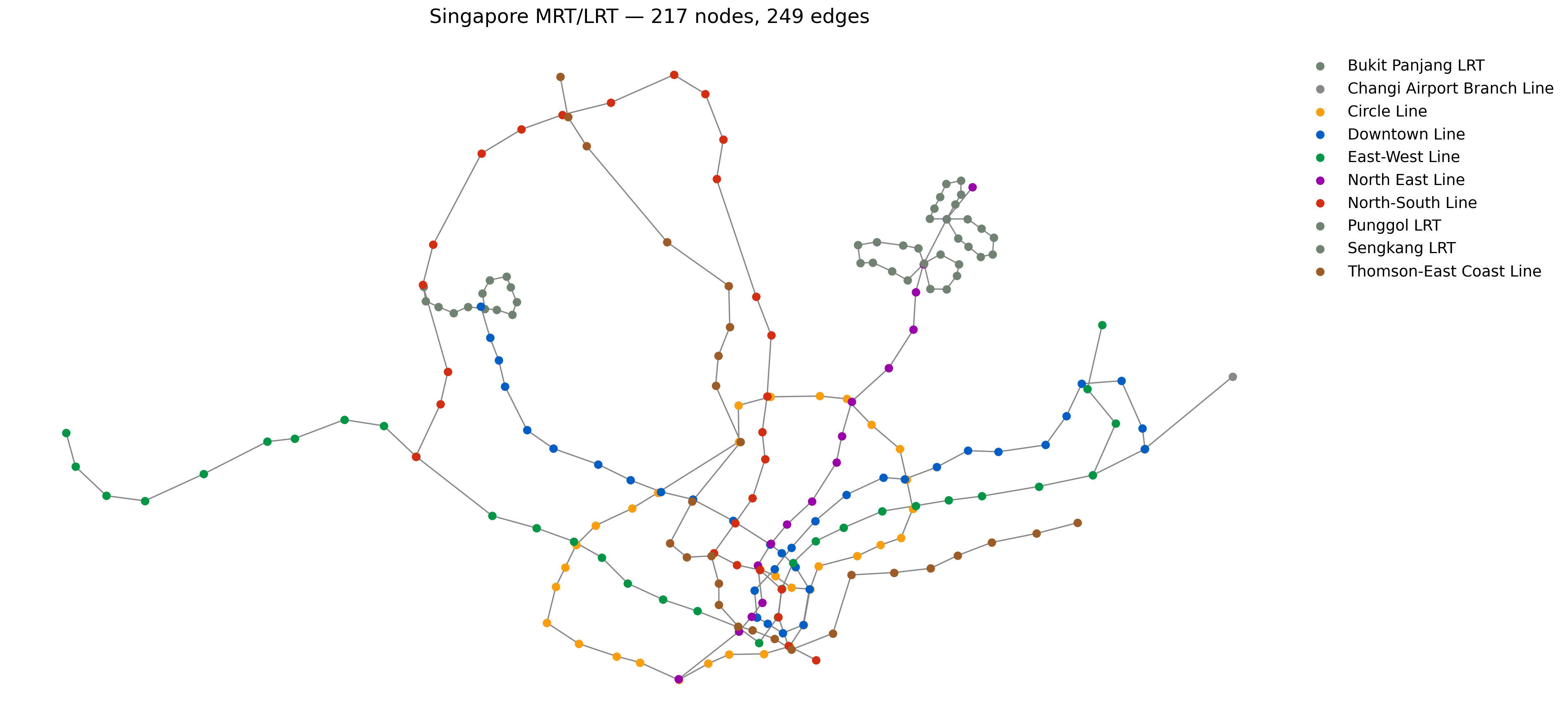
Make this Notebook Trusted to load map: File -> Trust Notebook

Figure 2: Singapore MRT/LRT network, stations coloured by line

Step 4: Add on travel times using GTFS schedule for realistic routing

Travel times between stations

To accurately assign passenger flows, an objective measure of how passengers might likely travel, given an origin, and destination station is needed.

A suitable measure is the total travel duration of the trip. Passengers desire to minimise travel times to their destination, and naturally select the fastest route between origin and destination stations. Passengers intuitively refer to Google Maps or Citymapper to find the shortest time taken to get between A and B, and so this is a representative way to model passenger behaviour and choice. Other options include optimising for physical track distance or travel cost, but both feature less prominently in the decision-making process. Moreover, Singapore adopts a distance-based charging approach to ensure that passengers are charged based on their actual usage of the transport network, so the difference in prices between different routes to the same destination is minimal.

To obtain the travel times between adjacent stations in the network, we can tap on the unified GTFS schedule provided by LTA via DataMall. While this can simply be obtained through the station boards encountered at station platforms, the GTFS schedule provides travel durations specific to train schedules at different periods of the day, which enables more accurate modelling.

Travel time information commonly found on station boards. Source: SBS Transit

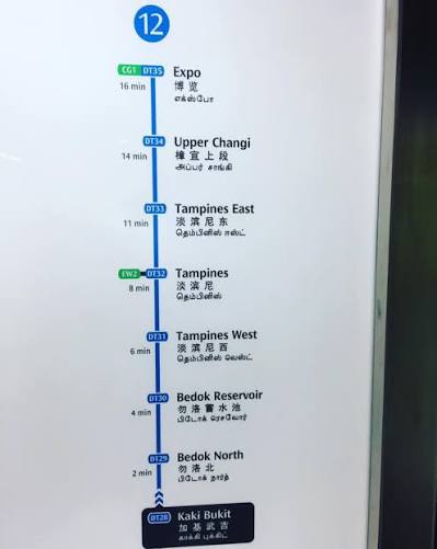
Understanding GTFS schedule data

GTFS (General Transit Feed Specification) is the standard format agencies publish timetables in. Two parts matter:

• Routes and stops: A stop is a place passengers board, and a route is a named service (e.g. the East-West Line). A trip is one vehicle running that route once, and stop times record when it calls at each stop in order — so the station sequence comes from the timetable itself rather than from a map.
• Schedules and frequencies: Departures are given either as explicit clock times for every trip, or as a headway — one trip every few minutes between set hours.

In Singapore, this data comes from LTA DataMall, which aggregates travel time information across the major operators SMRT and SBS Transit. The GTFS describes the planned timetable, not observed operation.

Time taken for interchange transfers

Another piece of information needed to construct an accurate network is the time taken for transfers at interchange stations. Singapore has approximately 30 train interchange stations. However, not all interchanges were built the same. Earlier ones like City Hall and Raffles Place were constructed with transfers in mind with platforms opposite each other or one short escalator ride away. Newer interchange stations like Bugis, Buona Vista and Woodlands require passengers to walk longer distances for connecting trains. Fortunately, we have this data courtesy of Reddit user u/catcourtesy, who measured each transfer timing between platforms of different lines by walking through the actual transfers. In reality, transfers also include the waiting time for the train on the next line. To account for this, 3 minutes were added on average for all transfers.

Shortest total travel duration

By combining travel time between stations and transfer times within interchange stations, a realistic graph network for the MRT/LRT system can be built. Dijkstra’s algorithm was applied to find the shortest path between two stations, which can then be used to derive the most rational route with transfers, and allocate passenger flows between origin and destination stations accordingly.

The table below shows an example of an optimal route taken between Tampines (DTL) and Bishan (CCL).

Shortest journey from Tampines (Downtown Line) to Bishan (Circle Line): 1 transfer, 11 stops, about 29.2 minutes.

Station	Name	Line	Time (min)
DT32	Tampines	Downtown Line	0.0
DT31	Tampines West	Downtown Line	2.0
DT30	Bedok Reservoir	Downtown Line	4.0
DT29	Bedok North	Downtown Line	6.0
DT28	Kaki Bukit	Downtown Line	8.0
DT27	Ubi	Downtown Line	10.0
DT26	MacPherson	Downtown Line	13.0
CC10	MacPherson	Circle Line	17.2
CC11	Tai Seng	Circle Line	19.2
CC12	Bartley	Circle Line	21.2
CC13	Serangoon	Circle Line	23.2
CC14	Lorong Chuan	Circle Line	26.2
CC15	Bishan	Circle Line	29.2

Table 3: Shortest journey from Tampines (Downtown Line) to Bishan (Circle Line): 1 transfer, 11 stops, about 29.2 minutes.

Step 5: Allocate Origin-Destination Passenger Flows

Next, we allocate the origin-destination (OD) passenger volume data. Data from LTA covers the number of trips between MRT stop pairs, where passengers tap in and out of the fare gantry. Trips are reported by hour and by day type — weekdays, and weekends/public holidays. Each OD pair’s trips are then assigned to the fastest path between its endpoints, and every edge along that path is credited with them.

For the purposes of this annex, Weekday AM peak (7–9am) flows were used from Aug 2026.

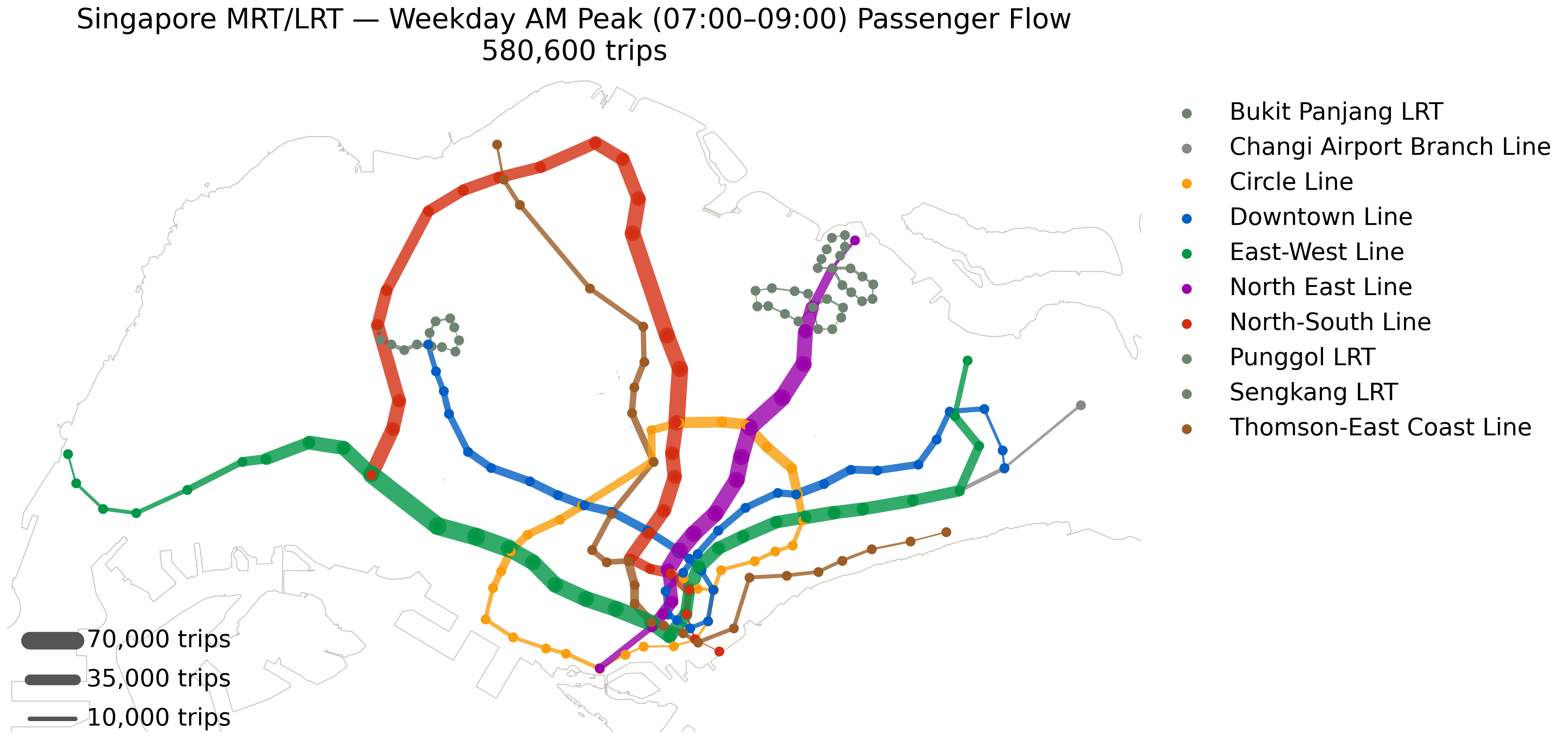
To visualise the flows, a graph of Singapore’s MRT and LRT system was plotted, with edge thickness corresponding to passenger flows during the weekday AM peak. Because the graph is undirected, each edge carries the combined load in both directions. On this measure, the heaviest loading sits on the East-West Line’s western approach, Jurong East to Clementi, Clementi to Dover and Dover to Buona Vista, followed closely by the North East Line through Hougang to Kovan and Kovan to Serangoon.

That ranking changes once direction is taken into account. The North East Line shows stronger tidal behaviour. Kovan to Hougang carries roughly nine times as much traffic inbound as outbound during the morning peak, against a little over three times on Dover to Buona Vista, possibly due to the counter-flows from Buona Vista’s employment cluster. Ranked by peak-direction load rather than two-way total, the North East Line segments move to the top.

Figure 3: Passenger link loads on an average weekday during the 7–9 AM peak. Line thickness is proportional to the number of trips whose fastest route traverses that segment; dotted lines are interchange transfers.

Table 4: Busiest track segments by combined two-way load, average weekday AM peak (07:00–08:59).

Busiest track segments by combined two-way load, average weekday AM peak (07:00–08:59).

From	To	Line	Both ways	Peak direction	Peak share
Dover	Buona Vista	East-West Line	71,376	52,174	73%
Clementi	Dover	East-West Line	71,126	53,265	75%
Jurong East	Clementi	East-West Line	70,339	52,358	74%
Kovan	Serangoon	North East Line	68,148	60,141	88%
Hougang	Kovan	North East Line	63,957	56,837	89%
Ang Mo Kio	Bishan	North-South Line	63,838	53,180	83%
Farrer Park	Little India	North East Line	63,518	56,159	88%
Tiong Bahru	Outram Park	East-West Line	63,065	41,995	67%
Woodleigh	Potong Pasir	North East Line	62,150	54,987	88%
Boon Keng	Farrer Park	North East Line	61,993	55,144	89%

Table 5: Busiest track segments by peak-direction load, average weekday AM peak (07:00–08:59). Direction shown is the busier of the two.

Busiest track segments by peak-direction load, average weekday AM peak (07:00–08:59). Direction shown is the busier of the two.

From	To	Line	Peak direction	Reverse	Peak share
Kovan	Serangoon	North East Line	60,141	8,007	88%
Hougang	Kovan	North East Line	56,837	7,121	89%
Farrer Park	Little India	North East Line	56,159	7,359	88%
Boon Keng	Farrer Park	North East Line	55,144	6,848	89%
Woodleigh	Potong Pasir	North East Line	54,987	7,163	88%
Potong Pasir	Boon Keng	North East Line	54,809	7,005	89%
Serangoon	Woodleigh	North East Line	54,439	7,386	88%
Clementi	Dover	East-West Line	53,265	17,860	75%
Ang Mo Kio	Bishan	North-South Line	53,180	10,658	83%
Little India	Dhoby Ghaut	North East Line	52,880	7,187	88%

Likewise, we can plot these flows corresponding to each hour of the day and see how the thickness of the edges vary. Notice how the flows change quite significantly with bimodal AM and PM peaks.

Figure 4: Weekday passenger link loads by hour of day.

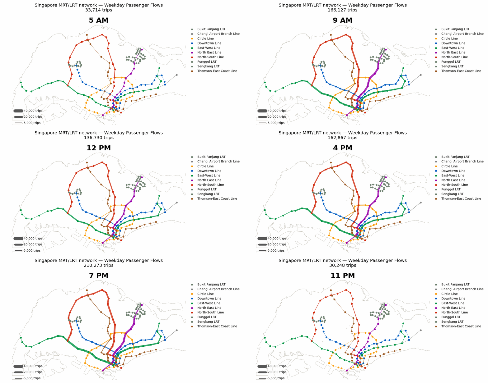
This pattern illustrates the persistent challenge for infrastructure planners all around the world dealing with bimodal peaks. Capacity needs to be adequately provisioned for the heaviest direction in the heaviest hour, yet overall network usage remains noticeably lower for the rest of the day, often making it difficult to justify the disproportionate capital and operating expenditure needed to sustain a larger network. Addressing this challenge requires a concerted effort with a range of different measures such as staggered working hours, off-peak fare incentives, and careful land use planning that distributes trip origins and destinations more evenly across the network.

Now, we are ready to move on to deeper investigation and analysis.

This article was written in tandem with coursework for the CASA0002 Urban Simulation module.

References

Barabási, A.-L. (2025) Network Science by Albert-László Barabási. Available at: http://networksciencebook.com/ (Accessed: September 10, 2026).

CNA (2026) “Blending form and function: A first look at 3 new MRT stations that will close the Circle Line loop - CNA,” Channel News Asia. Available at: https://www.channelnewsasia.com/singapore/circle-line-cantonment-price-edward-road-keppel-mrt-stations-first-look-6172836 (Accessed: September 10, 2026).

GeekforGeeks (2026) “Find Shortest Paths from Source to all Vertices using Dijkstra’s Algorithm,” GeeksforGeeks. Available at: https://www.geeksforgeeks.org/dsa/dijkstras-shortest-path-algorithm-greedy-algo-7/ (Accessed: September 10, 2026).

LTA (2015) “Train Station Chinese Names LTA data.gov.sg.” Available at: https://data.gov.sg/datasets/d_d312a5b127e1ae74299b8ae664cedd4e/view (Accessed: September 10, 2026).

LTA (2026) “LTA Dynamic Datasets.” Available at: https://datamall.lta.gov.sg/content/datamall/en/dynamic-data.html#Public%20Transport (Accessed: September 10, 2026).

NetworkX (2025) “NetworkX — NetworkX documentation.” Available at: https://networkx.org/en/ (Accessed: September 10, 2026).

OSM (2026) “Singapore/Rail Transport - OpenStreetMap Wiki.” Available at: https://wiki.openstreetmap.org/wiki/Singapore/Rail_Transport (Accessed: September 10, 2026).

URA (2026) “Master Plan 2025 Planning Area Boundary (No Sea) URA.” Available at: https://data.gov.sg/datasets/d_2cc750190544007400b2cfd5d7f53209/view (Accessed: September 10, 2026).